Understanding Market Cycles to improve your Stock Market Trading

A cycle is a chain of events that repeats over time. The outcome might not be the same each time but the characteristics are quite similar. Take for example the four season weather. Each year we have spring, summer, autumn and winter. After winter we have spring again and the cycle of weather will begin anew itself again. However this year’s summer will not be the same as last summer as the temperature varies every year.

Cycle frequencies can both be short and long, it can last from minutes until thousands of years. Understanding long term cycles in stock market helps you determine the overall market trend and similarly short term cycles helps you determine your timing in the entry and exit points in the stock market. The following chart shows some short and long term cycles.

Perhaps one of the most extensive studies on cycles is done by Dr Raymond H. Wheeler, Chairman of the Department of Psychology, University of Kansas. He commissioned 200 researchers to work for 20 years to study the effect of weather on mankind and also cultural activities dated back to the dawn of civilization. Over 3000 years of weather pattern was studied and so was 20,000 pieces of art and literature. After the extensive study he concluded that there exists a 100 year climate cycle and phases that influence human behaviours. The different phases can be described as the following:

1. Cold-Dry
2. Warm-Wet
3. Warm-Dry
4. Cold-Wet

510 years World Dominance Cycle

According to his calculations we are now in the Warm-Wet phase and should last until 2100. Further to this he also discovered the 510 years world dominance cycle. His record dates back 3000 years ago during the Greek and Roman eras. The following are dates and events that took place since then.

1. 570 BC - The Romans came to power after the Greeks collapsed

2.  60 BC - The Romans weakened and gave rise to the emergence of Asian Powers

3. 450 AD - Asian Powers declined and gave rise to Charlemagne and Britain power

4. 960 AD - Global power shifted back to Asia with the rise of Genghis and Kublai Khan.

5. 1470 AD - Europeans at the forefront of global dominance. Spain and Portugal were at their height of power when their naval fleet reaches the four corners of the Earth. Later we also see the re-emergence of Britain and also other European powers like The Netherlands and Germany. The United States came into the scene at a much later stage when the Global Power is about to be shifted back to Asia.

6. 1980 AD - As can be seen since 1980 the shift in the Global Power from West to East began once again. Since the 1980s we can see the re-emergence of Asian powers like China, Russia and India. So once again the balance of power will stay in the East for the next 510 years which will go right into the year 2490.

The above are extracts from Dr Raymond’s book called ‘The Big Book’ which contains most of his cycle studies. In it you will find that the 510 year ‘civilization cycle’ can further be broken down to three 170 year cycles which itself contained three 50-56 years cycles and so on. In other words there are cycles within a cycle. The most famous economic cycle is the Kondratieff Cycle (50-54 years). Kondratieff, a Russian economist whose cycle study is based on wholesale prices, interest rates, wage levels and production indexes from the period 1780 to 1920. In his paper titled ‘The Long Waves in Economic life’ he showed that there is an existence of a 48-60 years cycle in the overall economic activity in the Western world. The following chart shows the Kondratieff wave in action in the U.S Stock market.

Where are we now?

Historians have found that 50 years business cycle has already been in existence since the biblical days. In the Old Testament it did mentioned about farmland being lie fallow in the seventh year of cultivation. After a total of seven groups of these seven years (7x7 = 49 years) the land was to lie fallow two years in a row. The main question is where are we now in the Kondratieff cycle? From his study on economic cycles he found that the most valid recent peaks are occurring in 1814, 1865, 1929 and 1974s and the next peak will be around 2020s. The 50 years Kondratieff cycle can be classified by the following phases which are divided into five equal decades.

1. First Decade – Recovery (1974-1984)
2. Second Decade – Boom (1984 – 1994)
3. Third Decade – Peak and Transition (1994 – 2004)
4. Fourth Decade – Collapse (2004 – 2014)
5. Fifth Decade – Trough and transition (2014 – 2024)

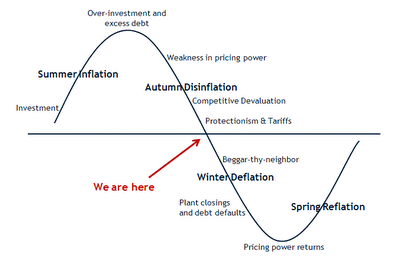
We reckoned that we are now in the fourth decade of the main cycle because currently global economies are engaging in competitive currency devaluations and also at the same time enacting protectionism policies. The following graph shows a more detailed succession of events leading to the current situation and also what to expect from now on.




Does a Stock Market Cycle exist?

Edward R Dewey can be considered the modern day authority in cycle studies. In his book ‘Cycles’ he documented his studies on cycles with data dating back to the 1830s. His book is considered the bible of cycle studies as to Benjamin Graham’s Security Analysis to Fundamental Analysis. What he found that the 9.2 or 9.225 years cycle to be exact is the most accurate of all. He estimated that there is only 1 in 5000 chance that the occurrences can be coincidental. 

Then we have Veryl L. Dunbar in his 1947 article ‘The Bull Market’ printed in Barron’s June 1952 issue discovered the 46 month cycle. His analysis on cycles for the past 123 years yielded a 97% accuracy rate or predicted 62 out of the 64 cycle occurrences. John Hurst, another pioneer in cycle studies identified 12 dominant cycles existing in the stock market. Below we present to you a table of compilations of various cycles and different timeframes of the stock market that has existed and still valid till today although there might be some slight changes in the timeframes.

Years	Months	Weeks	Days
18
9
4.5
3
1.5	18
1	12
0.75	9
0.5	6	26	182
0.25	3	13	91
	1.5	6.5	45.5
	0.75	3.25	22.75
	0.375	1.625	11.35
	0.1875	0.8125	5.687
	0.0937	0.4062	2.843

How cycles can assist you?

As a Stock Market investor would it be nice to add a tool to your arsenal that may help you to determine the general trend of the market and also to buy or sell before the market reverses. As you know Stock Market prices move in trends either up, down or sideways. For long term investors (defined as holding stocks more than 1 year), a solid knowledge of long term market trend or cycles is sufficient. This is also known as the Primary Trend in the Dow Theory.  

For medium term investors who are holding their portfolio between three weeks to a year, it will be advantageous to have some knowledge of the Secondary Trend or cycle. Secondary Trend refers to stock market trends that last between 3 weeks to a year. Lastly for short term investors who are likely to hold stocks for not more than 3 weeks again it will be advantageous to have some knowledge of the Minor Trend or cycle in the stock market. The following chart represents a cycle in the form of a sine wave. It also shows the different stages of market activity in one market cycle. During the trough stocks are accumulated and will be mark-up on the way up. At the peak stocks will be distributed and when done then it’s time to mark-down their prices and the cycle will begin anew again.

We will demonstrate to you using a live sample with the FBMKLCI. The following chart of the FBMKLCI clearly exhibits the existence of cycles. There are two cycles in existence and the first is between October 2012 and December 2012 while the second starts from the beginning of December 2012 to Mid February 2013.

If you have bought during the first low during the end of November 2012 and also the second low in mid February 2013, we are confident that your investments will performed much better than other times during those periods. So we hope that by now you should realised that with a clear understanding on market cycles and trends it will certainly help you make better informed decisions in your stock market investments.

Relationship between Current U.S deficits, Exchange Rates and Triffin's Dilemma

After the Great Depression in the 1930s the state of affair of the World economy can be at best described as turbulence.  As a result of the Great Depression many countries experience a period of plummeting personal income, tax collection, exports and consumption. During that time most of the world’s economies have unstable exchange rates which also resulted in unstable world trade. Following this many countries engaged in competitive currency devaluation which resulted in the ‘beggar thy neighbour’ policies being adopted. Hence due to the intensified currency wars among nations ‘protectionist’ trade policies are also introduced.

Bretton Woods System

By protectionist policy we meant setting up of artificial trade barriers like increased import duties, subsidies for so called ‘infant and export oriented’ industries and setting of quotas among nations. This is the exact opposite to free trade which promotes the smooth flow of international trade without any barriers. The situation had gotten worse and as a result there was a call for a new International Monetary System. In July 1944, delegates from 44 countries gathered at the United Nations ‘Monetary and Financial Conference’ in Bretton Woods, New Hampshire. There are two main agenda that are discussed during the Conference which is to introduce a new international financial monetary system to stabilize the current currency woes and also on the recovery of Europe after the WWII to prevent any recurrence of the problem.

Under the Bretton Woods system member countries are required to peg their currencies to the dollar and are allowed to fluctuate within a fixed trading band and also permitted to convert their dollar holdings to gold at the rate of $35 an ounce.  It is only the natural thing to do because during that time the US economy is accounted for almost half of the global manufacturing capacity and also holds the world’s largest gold reserve.  To facilitate the changes in the monetary system two international institutions are formed and they are the IMF (International Monetary Fund) and the World Bank. Apart from providing loans for the reconstruction of Europe post WWII it is also hope to stabilize the currency fluctuations so as to avoid future currency wars again. However over the long term such arrangement proved cumbersome due to the changes in the currency’s purchasing power parities (PPP).

Purchasing Power Parity

PPP refers to the value of basket of goods in two countries should be equal to the ratio of their exchange rates. For example if the exchange rate between the USD/MYR is 3.20 then a basket of goods consist of chicken, beef, eggs, flour, sugar and cooking oil that costs US100 in the U.S then the same basket of goods should be worth RM320 in Malaysia.  However such scenario will not often played out as expected due to both traded and non-traded inputs.

A good example will be the Big Mac index which is developed by the Economist illustrates the difference in the PPP of different countries. By definition a Big Mac cost US4.20 in the U.S should costs RM 13.44 (US4.20 x 3.2) in Malaysia. A check at a McDonald’s restaurant in Malaysia reveals that a Big Mac only cost RM 7.95 and convert it to US dollars it will translate to (7.95/3.2 = 2.48) US 2.48. This represents a (US2.48/US4.2) 59% discount in pricing on the Malaysian side. So in theory based on the PPP the Malaysian Ringgit is 59% undervalue and in the long run should appreciate upwards until it reaches parity with the USD. The full extent of the Big Mac Index can be shown in the following.






On the left are countries whose currencies are undervalued while those on the right are overvalued. The difference in currency values are attributed to both tradable and non-tradable inputs. In less developed countries certain goods and services such as labour and raw materials are cheaper and hence the end product in this case a Big Mac will be cheaper.  So as you can see the imbalances in the purchasing power parity of the different currencies will somehow has to move towards a more equitable level in the future.

One of the solutions will be the arbitrage of labour and resources through Foreign Direct Investments (FDI). Through FDIs companies from more developed nations are able to take advantage of the availability of cheap labour and resources in less developed countries. Furthermore FDIs will also help to reduce the currency imbalances when foreign companies convert their currencies to the local currency.

Triffin’s Dilemma

So coming back to our discussion on the exchange rates between countries under the Bretton Woods system, there will be parity problems because they are pegged to the USD. Member countries are not permitted to meddle with their exchange rates and hence as a result some of them are burdened by either their overvalued or undervalued currencies.  Without the ability to adjust their exchange rates countries will find it very difficult to achieve both internal and external balance. Sooner or later the currency peg under this system will be under tremendous pressure and eventually will have to give way.  In 1959 Robert Triffin also known for his (Triffin’s Dilemma) warned that the Bretton Woods system cannot survive because in order for the dollar to be continued as ‘the world reserve currency’ it had to supply more dollars and run ever bigger deficits.

The mechanics of it can be explained by the following. When the USD becomes the World’s reserve currency it will be the currency of choice by the world’s central banks when they build up their foreign reserves. Due to the popularity of the USD and hence an ever growing demand for it the value of the USD will keep appreciating. When a currency appreciates it will be cheaper to import and expensive to export. Hence as a result the deficits will be growing larger over time.  

However the growth of Money Supply in the Unites States seems to be on an exponential path as shown by the chart below. As with anything when the supply exceeds demand its value will have to drop. 




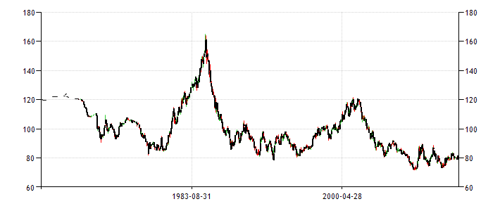
The following chart shows the United States Dollar index whose performance is measured against a basket of other currencies such as EUR, JPY, GBP, CAD, CHF and SEK. As can be seen its value seen tumbling since the 1980s which is also coincide with the increase in the money supply during that period then.



Source : Trading Economics


Bretton Woods and Fractional Reserve Banking

The Bretton Woods system operates in a similar way as the ‘Fractional Reserve’ system operates by the Banking industry. In the banking system deposits are used to leverage the bank’s ability to lend. For every dollar deposited the bank is able lend out more than $10 after allocated a certain amount for the deposit reserve ratio. It will be safe as long as all the depositors will not concurrently demand cash for their deposits. In other words when there is no ‘bank run’.  Similarly in the Bretton Woods system it is dealing with Gold and USD. The member countries (holders of USD) were given the impression that there is enough gold for everyone. However Triffin realized that as time goes by the amount of trade between countries will grow and hence the demand for USD will also increase. The problem is that there will come a time when the total dollar holdings by foreign central banks will exceed the amount of gold held by the United States.  

What will happen if foreign holders of USD simultaneously convert their USD holdings to gold at $35 an ounce? This is exactly what happened during the late 1960s. During that time the balance of payment deteriorated badly and there are fears of the Dollar devaluation. As a result many foreign holders of USD began to cash in their dollars for gold. This trend grew so fast and substantial where the U.S gold stock reduced by almost 70%. In other words there is a ‘Gold Run’ going on. So to prevent further depletion of its Gold Reserves, President Nixon on August 15th 1971 announced that foreign dollar holders are no longer able to convert their dollars to Gold.  Hence the USD is no longer backed by Gold and instead it is transformed into the ‘reserve currency of the world’ and is ‘backed by full faith and credit of the United States’. This brought an end to the Bretton Woods system and later the USD is allowed to ‘float’ with other currencies.

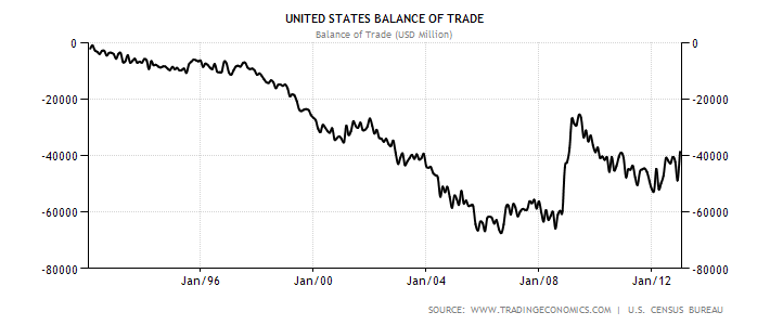
Nevertheless the deficits still remained after more than 30 years since then. The following chart shows the extent of the U.S deficits since the 1980s.



The reason why the United States is able to run deficits for more than 30 years is mainly due to the status of the dollar as the reserve currency of the world. Foreign central banks are obliged to keep their foreign reserves in dollars as it is also the currency of trade. Most commodities like oil, gold, corn, wheat and etc are quoted in dollars. Whenever a foreign country exports to the United States it will be paid in dollars. Those dollars will make its way to the foreign central bank which in turn will be recycled back to the United States in the form of purchase of dollar denominated assets or U.S Treasury Bills. Or they can add it to the foreign reserves. Can you notice there is a dilemma here? As time goes by the amount of USD accumulated by foreign dollar holders will multiplied and it is not in their interest to see the dollar ‘race towards zero’. If the dollar losses more value then naturally the value of their dollar holdings and dollar denominated assets will also go down. Put it another way the foreign dollar holders are trapped.


So are there any solutions available?

The first measure available to dollar holding countries is to stop adding more dollars to their reserves but instead diversify their future holdings of foreign reserve in other currencies such as the Euro or the Japanese Yen.

The second measure to counter the depreciating value of the USD is to trade using other currencies or even gold. Malaysia has already set several precedents when it paid the Chinese Government with palm oil for their work and finances in a railway project and also with Russia when it purchased some MIG fighter jets. In fact many countries have already started trading bypassing the use of dollar. India announced last month that it will begin to buy oil from Iran with gold and not dollars. On September 2012 China also announced its intention to sell oil denominated with the Yuan. So as you can see the exodus from dollar denominated trade is gaining speed and sooner or later the USD is going to lose its importance as the world’s reserve currency.  
 

Is Malaysia's Economy heading for Bankruptcy in 2019?

Malaysia can be considered a success story in terms of economic development. It successfully transformed itself from being a backwater undeveloped economy to a middle income country. It manage to do that by transforming its resource based to a manufacturing economy and also able to reposition its economy by attracting much of the Foreign Direct Investments during the 1970s and 1980s. Transfer of technology and also modern managerial skills that are brought about by the Multinational Corporations (MNC) also helped build up our pool of skilled labours which in needed in our economic transformation in the later years. Due to the transformation and repositioning of our economy it also altered the importance of certain sectors of the economy which is shown in both the composition of its exports and imports.

Our exports are now consists of electrical and electronics – 35%, palm oil – 15%, petroleum products – 9%, LNG – 7% and the rest are made up of timber, various manufactured goods and etc. Our imports are mainly made up of machinery and transport equipment – 60%, manufactured goods – 12%, fuel - 10% and chemical - 9 %. The interesting thing to note about Malaysia’s imports is that the bulk of it are made up of ‘Capital Goods’ and not consumer items such as food, beverages and etc.  When a country imports more capital goods than anything else it shows that this country is on the right track to a ‘sustainable developing’ economy because these capital goods such as machineries and transport equipment will be used to furthered the production of manufactured goods and hence helped promote economic growth.

Government watering our wages?

Below we present to you several development and income metrics of the Malaysian Economy which we hope to help you understand where our money gone and also why our ‘income distribution’ is not catching up with the system. We hope you can bear with us as it is quite statistical and boring.

The macroeconomic metrics we used are the following:

1. Wages in Manufacturing
2. Malaysia GDP
3. Wage/GDP index
4. Malaysia Government Debt/GDP
5. Malaysia Money Supply M3
6. Malaysia GDP per capita
7. Malaysia Government Spending
8. Malaysia Consumer Spending
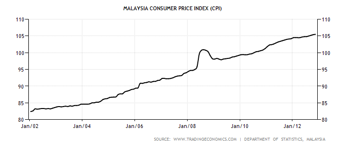
9. Malaysia Consumer Price Index
10. Malaysia Government Budget

Later we will also show the inability of income to catch up with general price level of goods and services or inflation which is measured by the CPI. Hopefully it will also help us to answer the following question on whether the authorities are watering our worker’s wages?

Why our Income lagged GDP Growth?

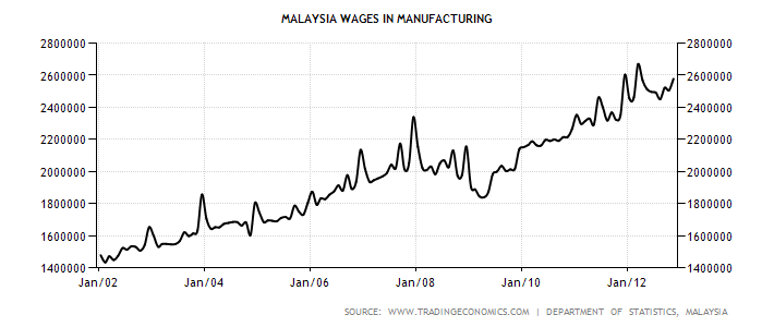
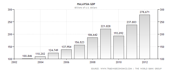
As far as we know there are not many papers written on this subject and reasons being the lack of interest or simply not reported in the mainstream media to avoid any troubles with the power to be. Anyway we present to you 2 charts on the wages in manufacturing and also the GDP growth of Malaysia as a basis for our comparison. Wages in manufacturing is selected because the manufacturing sector employs the most people in Malaysia.  



The following is a chart on the Manufacturing wages to GDP that we plot using data from the above wage and GDP charts. It clearly shows that the worker’s share of the GDP has certainly been dropping since 1999. So where have the bulk of the remaining GDP went?




Certainly not us and you folks! The main culprits are the Government and its unscrupulous cronies and capitalists. With the projected FBMKLCI earnings growth of 8.0 and 8.4% for 2013 and 2014 respectively, obviously things are looking good for the corporates ahead.  With an average earnings growth rate of 8% for the past couple of years while the ratio of Wages/GDP declining it is obvious that those bastard capitalists have been capping the increase in wages so as to maximise their profits. Since Malaysia’s competitive level has been declining, the question is how those companies are able to keep recording increasing profits?

Green Belt help creates scarcity

One explanation will be the effects of inflation and the other being the existence of so called ‘Green Belt’ industries. The term Green Belt originated in London during the 1930s where the periphery of land surrounding the city was accorded this status. Property developments are discouraged in this area by tough regulations so as to create what we call ‘scarcity’ in economics. The main reason is to control the amount of housing in this area so that property prices and rents will always be high because there are not many choices or alternatives to choose from. Another reason is to control the amount of people living in the city so that the city will be free from congestion, pollution and other social problems that are associated with increased population. In Malaysia we have our version of the Green Belt in Kuala Lumpur. It is located in the Bukit Bintang area and also known as The Golden Triangle. Rentals in this area are able to match those in other major cities around the world like Singapore, Taiwan, New York and so on.

Coming back to our discussion on Green Belt companies that are able to capitalize their strengths from scarcities that arises within their Industries. Due to the nature of granting licenses in Malaysia, it enable many companies virtually operate in a monopolistic manner. Economists call this type of behaviour ‘Rent Seeking’ which is common in Malaysia. Due to their Green Belt status like which commands scarcity, there are able to charge higher price to consumers at their whims and fancy. Take the Cable TV business as an example, there is only ONE company that has the license to operate this business. Due to scarcity and being the monopoly, consumers are left with one choice – take it or leave it. When they raised their prices last year subscribers have no choice but to succumb to their whims.

Similarly in the power generation business licenses are given to the so called IPPs (independent power producers) to generate electricity which in turn sold back at a much higher price to our national utility company (TNB). These IPPs are able to enjoy Green Belt status as there are ensured that the barriers of entry are high and TNB will have to buy whatever amount of electricity that are generated. As a result these companies are assured of big profits every year. Other companies that enjoyed Green Belt status are PLUS Highway, Petronas, Indah Water, Bernas, FOMEMA and many more. These companies are able to raise prices without attracting much competition from competitors due to their strength from scarcity.

Malaysia’s Government Debt/GDP had been stabilizing around the mean of 43 % up till 2009. However since the year 2010 it had shot up to 55.4 % and had been remaining above the 50 % since then.  This is attributed to the RM 67 billion that is raised during the 2009 period in respond to the 2008 Global Financial crisis which was used as a stimulus package.

This sudden upsurge coincides with the increased in the Government spending which is reflected by the record deficit of -7.4 % of GDP in 2010. The following chart shows the gradual increase in the Government spending which only accelerates in recent years.  Having a Debt/GDP of 52 % doesn’t mean we are in a comfort zone because when Ireland and Portugal defaulted their Debt/GDP is less than 70%. Further to this we cannot compare to Japan whose Debt/GDP is 211 % as of Nov 2012. We will explain shortly why Japan’s economy will not default even with such high level of debts.    

Government Pump Priming the Economy

Pump priming refers to efforts by the Government to inflate the economy by initiating policies that will help expand the economy and hence its activity. It is no secret that most Governments in the world today are artificially boosting their economy either by depreciating their currencies, creating trade barriers or simply embark on an expansionary monetary policy in order to achieve full employment. The world economy is currently facing an extremely challenging time ahead as most Western economies are contracting and what will happen next will be the inevitable ‘Currency Wars’. By this we mean sooner or later each and every country will have to compete with each other by devaluating their currencies so as to make their exports cheaper which will help create jobs. Side effects of currency wars are Global Central Banks will increase their efforts to protect their economies by printing more money, create tensions among nations, beggar thy neighbour and lowering of bond yields due to currency interventions will also help increase interest rate sensitive consumption.

To begin with Malaysia’s money supply had been steadily increased for the past few years. The following chart shows Malaysia’s Money Supply as of 2002 till 2012.


Malaysia’s total Money Supply consists of M0+M1+M2+M3 which can be divided into the following,

1. M0 which is the most liquid of all. This includes notes and coins in circulation and also assets that are easily convertible to cash.
2. M1 is the second group of the total money supply and this also includes M0. As of Nov 2012 it stands at RM 270.48 billion.
3. M2 refers to the short term time or fixed deposits in banks plus M1. As of Nov 2012 the total is RM 1.32 trillion.
4. M3 is the long term time or fixed deposits in banks plus M1 + M2. The total figure for M3 as of Nov 2012 stands at RM 1.34 trillion.

How much has our Money Supply Grown?

From the records above, our total Money Supply in January 2002 was RM 475 billion but it somehow managed to explode upwards to RM 1.34 trillion in November 2012. This represents an increase of about 268% for the period of 10 years. Whereas in the U.S during the same period from 2002 to 2012, the total Money Supply as measured by M2, grown from $ 5426.2 billion to $ 10408 billion. Period to period in percentage terms their Money Supply had only grown by 91.8% (10408-5426/5426). This can be shown by the following graph.



How indebted are our consumers?

Due to the improving economic conditions since the Global Financial Crisis in 2008, Malaysia’s GDP per capita has also been improving. Since 2002 the GDP/Capita has been rising from the low of US 3933.94 to US 5364.50. This can be shown by the following chart.



The rise in income has altered the consumer spending pattern. There is a macro shift in consumer spending from the traditional ‘needs based’ to a ‘wants based’. This means consumers are splurging on luxuries rather than necessities. Consumers are more willing to splurge on the latest hand phones, luxury handbags, ipads, fine dining, overseas travel and so on without ever giving it a thought. As a result of their addiction to spending they began to look for more avenues to raise cash like credit cards and personal loans and hence lead to an explosion in the consumer debt level. The following two charts shows the upward trend in their spending habits and also helped to explained the explosion of both the public and private sector debts.




The trend in consumer spending in Malaysia seems to be edging higher and higher with no end in sight. Thanks to the our Government’s earlier effort in promoting a consumer spending economy and at the same time relaxing the requirements to obtain loans so as to create a ‘loose money’ economy albeit there have been efforts to curb such practices recently . From the above chart consumer spending rose from RM 59300 million in January 2005 to RM 99812 million in September 2012 which represents a 68 % increase during this period. Government controlled medias have been telling folks that the economy is recovering and we are moving forward to better times. In reality our private sector is one of the most indebted in the region and their debt level can be considered ‘up to the eyeballs’.

The following chart is the household debt/ Disposable income of several countries and Malaysia is no doubt the leader among them.




Deteriorating External Sector

Malaysia’s receipts from exports are also down especially from the plantation sector following the decline of Global Commodity prices. As a result Malaysia’s external sector has also been affected. Palm oil price is at RM 2400 down from the high of RM 3820 in 2011 and similarly rubber prices remain low trading at less than RM 1000 compared to the high of RM 2160 in 2011. Hence there are less funds available for the Government to spend as a result it incurs deficits in its budget.

 

A budget deficit is a situation where the Government spends more than it received. From the above it seems that our Government had been running budget deficits since 1999 till today. To finance budget deficits normally there are three options available to the government and they are reducing public spending, increase taxation or borrowing. Given the current depressed economic scenario, increase taxation in the form of income and sales tax may place further burden to the already over stretched consumers in Malaysia.

Reducing public expenditure will be out of the question because it will entail slower economic growth and will be suicidal politically in the upcoming elections. The last option will be to borrow from abroad through issuing sovereign bonds to foreigners or to local institutions like EPF and so on. Thus this will further increase our debt burden and eventually will also increase our Government’s Debt/GDP. The problem with higher Debt/GDP is that interest will have to be paid and in this case to foreigners although their share represents about 25% of the total. This will represent a leakage in the economy and hence there will be less money circulating around our economy and will certainly affects the level of economic activity.

Nevertheless the main threat to the Malaysian economy is its debts although our Debt/GDP ratio has yet reached critical level. The lesson we must learn from the Global Financial Crisis during 2008 is that the majority of the countries that went bust had their Debt/GDP below 70%. Below is the Debt/GDP table of those countries that fell during the Crisis.

Table 1.  Eurozone Countries Government Debt/GDP

Column1	Column2	Column3	Column4	Column5	Column6
Country	2008	2009	2010	2011	2012
Cyprus	58.8	48.9	58.5	61.3	71.1
Iceland	28.5	70.5	87.8	92.8	99.2
Ireland	25.1	44.5	64.9	92.2	106.4
Portugal	68.3	71.7	83.2	93.5	108.1
Spain	36.1	40.2	53.9	61.5	69.3
Italy	103.6	106.1	116.4	119.2	120.7
Greece	105.4	112.9	129.7	148.3	170.6

Source : Trading Economics

Any Risk in Defaulting?

As can be seen from the above, Malaysia cannot rest on its laurel that its Debt/GDP (52.6 %) is within manageable level. We must know that in normal market conditions risk and reward follows a linear path and that means higher risk will be compensated by higher return. However during extreme market movements (during a crash) risk and reward will follow a non-linear path meaning higher risk will not be compensated with higher return. In a Micro level an individual investor’s perfectly diversified portfolio that consists of many stocks and other derivatives will not be able to withstand extreme market movements. Say for example a 10 % drop in the FBMKLCI will normally result in a bigger decline in his portfolio and hence the P&L. Similarly on a Macro level Malaysia’s well diversified economy will not be spared either if one or two of its crucial macroeconomic metrics such as exchange rates (drop susceptibly) or interest rates (sky rocketing) reacted negatively to big market moves.

Further to that even if they try to pre-empt any extreme market movements by stress testing their portfolio or economy will not work. Evidence during the 2008 crisis proved that even though the banking industry tried to stress test their robustness with Quantitative Finance Risk Management tools such as VaR (Value at Risk) and CrashMetrics, it proved that is not sufficient to overcome to severity of the Crisis. Without bailouts from the authorities many of them will not be around by now.   

In Summary

The other day I was reading some articles written by some of our local analysts saying that Malaysia will not face any risk of defaulting because of our strong fundamentals. Further to that they argued that we cannot compare Malaysia with Greece or Spain because they had a history of defaulting and Malaysia has never defaulted before. What denial !! But there is always the ‘first time’ and we must remember that the first cut is the deepest. Malaysia is able to escape much destruction on its economy during the Asian Financial Crisis back in 1998 because that Crisis was mostly confined within the South East Asian region albeit causing a few mini crashes here and there in Russia and South America. But what is coming soon is a different animal and it is on a Global scale. The fuse has already been lit by the recent Currency Wars.